Introduction
Optical invariants serve as invaluable mathematical representations encapsulating various optical parameters within an optical system. Despite the dynamic nature of optical components, these invariants remain constant, providing a stable foundation amidst fluctuating parameters. This consistency enables engineers and designers to navigate the complexities of optical systems with greater efficiency and accuracy.
During the design phase of optical systems, the utilization of optical invariants streamlines the process, facilitating rapid progress while mitigating the risk of errors in calculating optical parameters. By relying on these invariant expressions, designers can expedite decision-making and optimize system performance without sacrificing precision. This expeditious approach not only accelerates the design cycle but also enhances the overall reliability and functionality of the optical system.
In essence, optical invariants serve as guiding principles, guiding the design and optimization of optical systems with unparalleled efficiency and reliability. By leveraging these mathematical expressions, engineers can navigate the intricate landscape of optical design with confidence, achieving optimal results while minimizing errors and delays.
Historical Context and Development of Optical Invariants
The historical context and development of optical invariants trace back to the early days of optics, where scholars and scientists grappled with understanding the behavior of light and its interactions with optical elements. The roots of optical invariants can be found in the work of prominent figures such as Isaac Newton, who laid the groundwork for modern optics with his seminal work, “Opticks,” published in 1704.
Over the centuries, advancements in mathematics and physics facilitated deeper insights into the nature of light and its propagation through optical systems. However, it was the pioneering work of 19th-century physicists like Augustin-Jean Fresnel and Sir George Gabriel Stokes that paved the way for the formalization of optical invariants.
Fresnel’s contributions to wave theory and his development of the Fresnel equations provided crucial insights into the behavior of light at interfaces, shedding light on the principles governing reflection, refraction, and diffraction. Meanwhile, Stokes’ investigations into the polarization of light and his formulation of Stokes parameters expanded our understanding of light’s properties and paved the way for the quantification of optical phenomena.
The concept of optical invariants gained prominence in the 20th century with the advent of matrix optics and the development of the optical transfer matrix formalism by Karl Willy Wagner. This mathematical framework provided a systematic approach to analyzing the propagation of light through optical systems, allowing engineers to predict the behavior of light beams with unprecedented accuracy.
In the latter half of the 20th century, advancements in computer technology facilitated the application of optical invariants in ray tracing algorithms and computational optics, enabling the design and optimization of complex optical systems with remarkable precision and efficiency.
Today, optical invariants continue to play a crucial role in the design, analysis, and optimization of optical systems across a wide range of applications, from imaging systems and telescopes to laser systems and optical communication networks. As our understanding of optics continues to evolve, optical invariants remain indispensable tools for engineers and scientists seeking to unlock the full potential of light-based technologies.
There are 4 main invariants of optical systems:
- Lagrange-Helmholtz invariant for paraxial optics
- Abbe sine condition for high aperture systems
- Straubel invariant for illuminating optical systems with light pencils transformation
- Etendue invariant for illuminating optical systems with extended source
Lagrange-Helmholtz invariant

Fig 1 presents an optical schematic shown with the help of principal planes ℎ and ℎ′.
Symbols on the scheme:
- y and y′ are heights of object and image
- α and α’ aperture angles in object and image spaces
- n and n’ are indices of refraction in object and image spaces
In case of small angles and ray heights, the relation between these parameters is represented below.
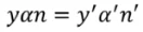
This is a well known invariant of Lagrange-Helmholtz. It shows that the product of aperture angle and field height is constant in image and object space. This relation works for any optical system with any number of optical components.
This invariant defines the relation between image aperture angle and image height when the object aperture angle and height are known and fixed. The main optical parameters of the optical system can then be defined.
In an existing optical system, Lagrange-Helmholtz makes it possible to estimate the relation between two pair parameters of object and image.
Modifications of Lagrange-Helmholtz invariant for different methods of object to image conjugation
Infinite to finite conjugation
Example: Objective lens of camera

Where ω is field angle, D0/2 is half of aperture diameter, F is f-number.
Infinite to infinite conjugation
Example: Galilean telescope system

Where ω is field angle, D0/2 is half of aperture diameter, F is f-number.
Lagrange-Helmholtz invariant application
Lagrange-Helmholtz invariant is very important for estimating the relation of parameters of systems in paraxial region, where apertures and fields of view are quite small.
This invariant defines the main parameters of paraxial optical systems: focal lengths, magnification, positions of object and image, entrance and exit pupil, and principal planes.
Abbe sine condition

Lagrange-Helmholtz invariant is true for any optical system with relatively small y (ω) and α. For an optical system where essential α is similar to a microscope lens, a more accurate invariant is needed, the Abbe sine condition.
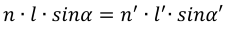
Comparison of Lagrange-Helmholtz invariant with Abbe sine condition shows that Sine condition uses the sinus of aperture angles instead of their values.
Abbe sine condition application
Sine condition is true for optical systems that don’t have spherical aberrations and coma. Vice versa, if sine condition is true for a given optical system, that system doesn’t have spherical aberration and coma. It is named aplanatic. In other words, sine condition is a condition of aplanatism. This is a key indicator of a microscope lens performance.
If the optical system has residual aberrations, this can be characterized as OSC (offense against the sine condition). The level of deviation from sine condition shows the extent of proximity of the concerned optical system to an aplanatic one.
One effect from sine condition is that the maximal aperture aplanatic systems is 0.5, though non achievable.
Light pencil invariant and Straubel theorem for transferring

Light pencil invariant and Straubel theorem for transferring
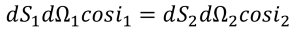
Let’s consider the propagation of a light pencil beam through the refractive surface (Fig. 5). The volume of a light pencil is limited by surfaces dS1, dS and the marginal rays between them. Two light pencil beams are presented on Fig. 5:
- Between dS1 surface and refractive surface dS
- Between refractive surface dS and surface dS2
Rays propagating between surfaces form several solid angles are dΩ, dΩ1, and dΩ2. The light pencil invariant demonstrates the interrelation of these angles and surfaces:
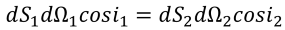
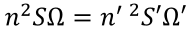
Straubel theorem takes into account the media refraction coefficient with different indices refraction n and n’.
This equation is valid for any number of reflections and/or refractions.
Etendue invariant

A real optical system works with extended sources with square n and finite apertures determined by the sizes and system construction. The light spot area generated by rays passed through the optical system is determined by the Etendue invariant:
where S and S’ are areas of source and its image and Ω is the solid angle which is defined as follows:
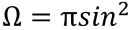
where u is aperture angle.
Accordingly, the Etendue invariant is:

Etendue invariant application
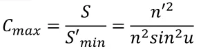
The limit of light spot size
We can use the Etendue invariant to find the ratio of source area and the light spot area formed with the help of optics.

The maximum value of sine function for the image aperture angle is 1 when the angle ?’=90°. In this case, the ratio will have a maximum value (Cmax). Its formula is:
Throughput of LED illumination optical system
If the optics are not large enough to overcome the source Etendue, there will be an additional efficiency loss. In this case,the source Etendue will be limited by optics Etendue; the Etendue invariant will not work. It can however help in finding loss levels and even in optimizing them with the help of this formula:

Need assistance designing a custom optic or imaging lens ? Learn more about our design services here.
Comparative Analysis of Invariants
The Abbe sine condition, Straubel invariant, and Etendue invariant are all fundamental concepts in optics, each addressing different aspects of optical systems. Let’s compare and contrast these invariants:
Abbe Sine Condition:
– The Abbe sine condition, named after Ernst Abbe, is a fundamental principle in optical design that governs the performance of optical systems, particularly imaging systems.
– It states that for an optical system to produce a diffraction-limited image, the numerical aperture (NA) of the system must be proportional to the sine of the acceptance angle of the marginal ray.
– The Abbe sine condition is primarily concerned with minimizing aberrations such as coma and spherical aberration, ensuring high-quality imaging performance.
– It is commonly used in the design of microscope objectives, camera lenses, and other imaging optics.
Straubel Invariant:
– The Straubel invariant, named after Carl Straubel, is a mathematical expression that characterizes the relationship between the object and image spaces in optical systems.
– It describes the conservation of optical path length between corresponding points in the object and image spaces, regardless of the specific configuration of lenses or mirrors in the system.
– The Straubel invariant is particularly useful for analyzing optical systems with complex geometries or non-linear paths, providing a means to assess image formation and distortion.
– It finds applications in fields such as optical metrology, where precise measurement and analysis of optical systems are essential.
Etendue Invariant:
– The Etendue invariant, also known as the conservation of étendue, is a principle in optical engineering that relates to the conservation of light flux or brightness within an optical system.
– It states that the product of the area and solid angle of light in the object space is equal to the product of the area and solid angle of light in the image space, assuming no losses or changes in divergence.
– The Etendue invariant is crucial for designing optical systems that efficiently collect, collimate, or focus light while preserving brightness.
– It is widely used in applications such as illumination systems, laser beam shaping, and radiometry.
Comparison:
– While all three invariants are fundamental principles in optics, they address different aspects of optical systems.
– The Abbe sine condition focuses on minimizing aberrations and optimizing imaging performance.
– The Straubel invariant relates to the conservation of optical path length and is useful for analyzing complex optical systems.
– The Etendue invariant concerns the conservation of light flux and is essential for designing efficient optical systems for various applications.
– Despite their differences, all three invariants contribute to the design, analysis, and optimization of optical systems, helping engineers achieve desired performance and functionality.
Conclusions
Optical invariants represent foundational principles that underpin the design, analysis, and optimization of optical systems. From the Abbe sine condition’s focus on minimizing aberrations in imaging systems to the Straubel invariant’s role in characterizing the relationship between object and image spaces, and finally to the Etendue invariant’s conservation of light flux, each invariant offers unique insights into the behavior of light within optical systems. By leveraging these invariants, engineers and scientists can navigate the complexities of optics with precision and efficiency, ultimately advancing technologies in fields such as imaging, metrology, and illumination.
Optical Invariants Explained: Frequently Asked Questions
What are optical invariants and why are they important in optical design?
Optical invariants are fundamental principles in optics that remain constant in an optical system under certain conditions. They are crucial for ensuring accuracy and efficiency in the design and analysis of optical systems, such as lenses and mirrors, as they guide the relationship between various optical elements.
How does the Lagrange-Helmholtz invariant apply to lens design?
The Lagrange-Helmholtz invariant relates the object distance, image distance, and refractive indices in an optical system. It’s particularly useful in lens design for determining the limitations and capabilities of a lens, such as magnification and light-gathering ability, ensuring optimal performance and clarity.
Can optical invariants be applied in modern digital imaging technology?
Yes, optical invariants play a significant role in digital imaging technology. They are used to design lenses and imaging systems that work efficiently with digital sensors, ensuring sharpness, proper light distribution, and minimizing aberrations in digital cameras and other imaging devices.